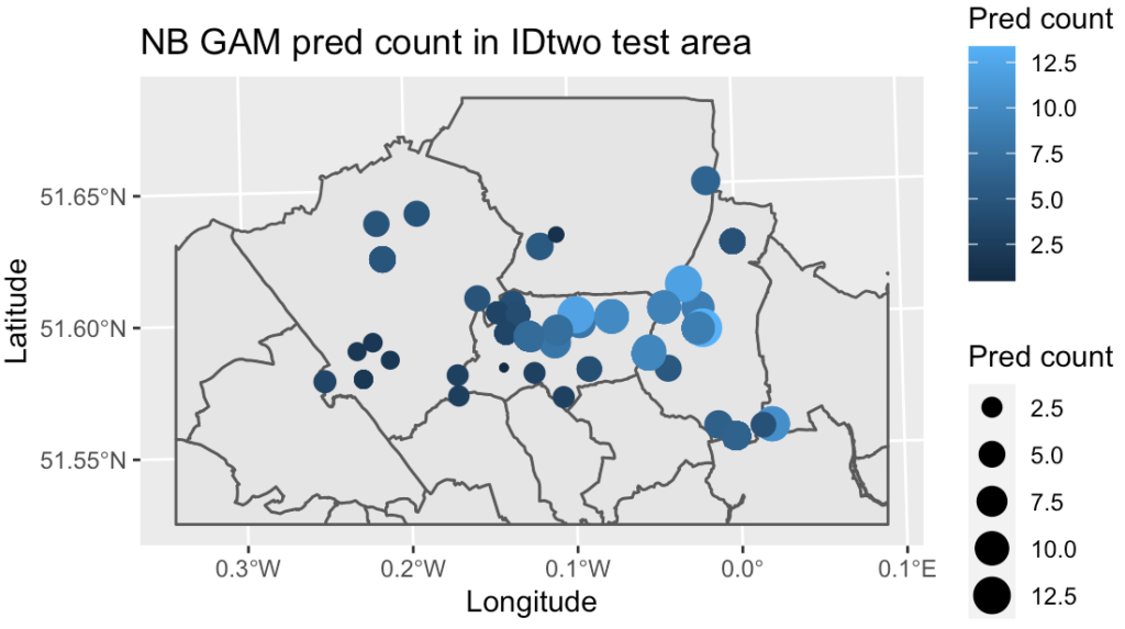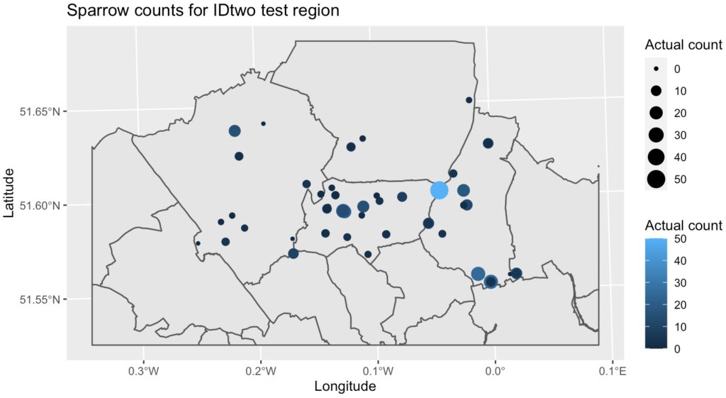
By analysing counts of species across a range of socio-environmental and climate variables, is it possible to model the count of house sparrows in a known urban area, and use these to predict likely numbers for a separate similar region?
This was the question I was seeking to answer as part of an MSc dissertation. I was interested in which variables affect populations of birds and whether they can be used to predict numbers of various species in a previously unmonitored area.
The house sparrow is one of the most globally-distributed species of bird. It’s also well adapted to living alongside humans in highly urbanised environments, ecologically tolerant and unbothered by human presence. So it’s often seen as a bioindicator species for the environmental quality and health of a local area.
The house sparrow
The last few decades have seen a significant fall in house sparrow numbers although there is no consensus on the specific reason. One study has suggested that house sparrow populations are not limited by food availability.
Observations or sightings are mainly opportunistic and carried out by bird enthusiasts and members of the public as well as expert bird watchers. Data was obtained under educational licence from Greenspace Information for Greater London (GiGL) and augmented with a separate dataset from the Global Biodiversity Information Facility (GBIF).
Data was cleaned to avoid missing entries or duplication, and the task of putting together a dataset of explanatory variables begun. A range of sources was used to create a dataset for 2018 for each of the Lower Layer Super Output areas across Greater London, and they included average temperature, rainfall, human population density, tree canopy cover, landcover type, and night light pollution.

The data was cleaned, merged, and split spatially into six geographic zones. Five of the zones were used as the training and validation dataset with the remaining region used a test set.
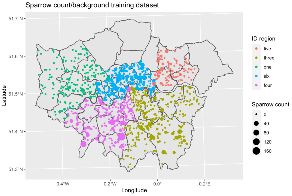
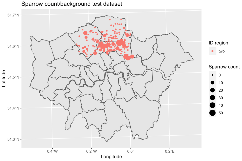
The Models
It is hugely challenging to fit and evaluate models to the data since biological ecosystems are complex. Although birds are an important bioindicator, being highly mobile, statisticians and ecologists have found that they are a tricky species to model. One flexible method used for different environments and animal species is Species Distribution modelling (SDM).
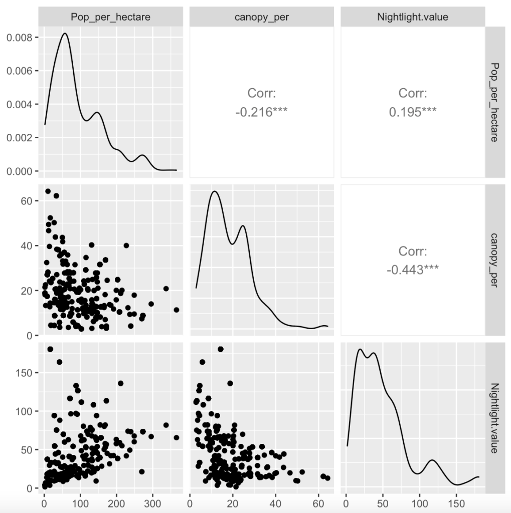
After exploratory analysis was carried out, which helped to reduce the number of explanatory variables, a range of models were fitted to the training dataset using R. The Poisson Generalised Linear Model (GLM) is generally the starting point for count models, followed by a negative binomial GLM, which is potentially provides a better fit where data is overdispersed. Generalised Additive Models were also fitted to allow Poisson and Negative Binomial distributions for the random part of the model. However the systematic element of GAM is a function rather than a coefficient for each variable, allowing greater flexibility in describing relationships. Machine-learning models using a random forest method were also developed.
Once models were obtained using the training data, they were run against the test dataset to find those that performed best.

The Results
Fitting a wide range of different models means they can’t easily be compared but different models can give clues as to which variables could be more important than others. Coefficient comparisons for GLM models and importance tables for the random forest models suggest that night light pollution, human population density, tree canopy and mean temperature could be the most important variables for predicting sparrow counts.
Intuitive relationships between variables are also revealed for example as night light pollution and human population increase, sparrow count is expected to fall. Surprisingly, as tree canopy levels increase numbers are predicted to fall, however this may be because the house sparrow fares better in urban gardens and hedges than in forested areas.
The random forest classification model gave an accuracy of 81% on the training but fell to 29% on the test set, indicating overfitting or an incorrect threshold level.
Conclusions
The Poisson GLM shows the data is overdispersed. A dispersion of 10.5 substantially underestimates the standard errors and renders this model unreliable for prediction. The negative binomial GLM allows variation in variance giving improved residuals and making more reliable predictions.
However, the predictive power of this model is low and it appears there are more complex, non-linear relationships at play between the explanatory variables and the response, and the GAMs appeared to be better at explaining the relationship. The Poisson GAM explained 74% of the deviance and 67% adjusted R2, but was still overdispersed. The NB GAM had a better root mean square error on the test set and more realistic count predictions, and so was selected as the best model to move forward with. Additionally the random forest classification model had a high accuracy but the maximum sensitivity/specificity threshold levels need further tweaking.
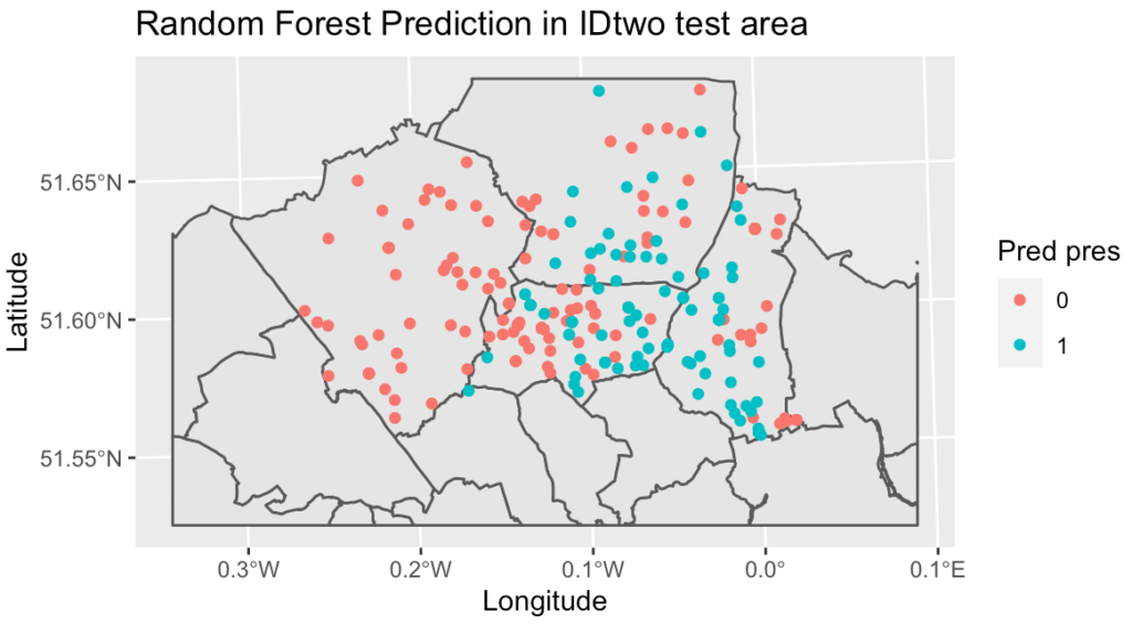
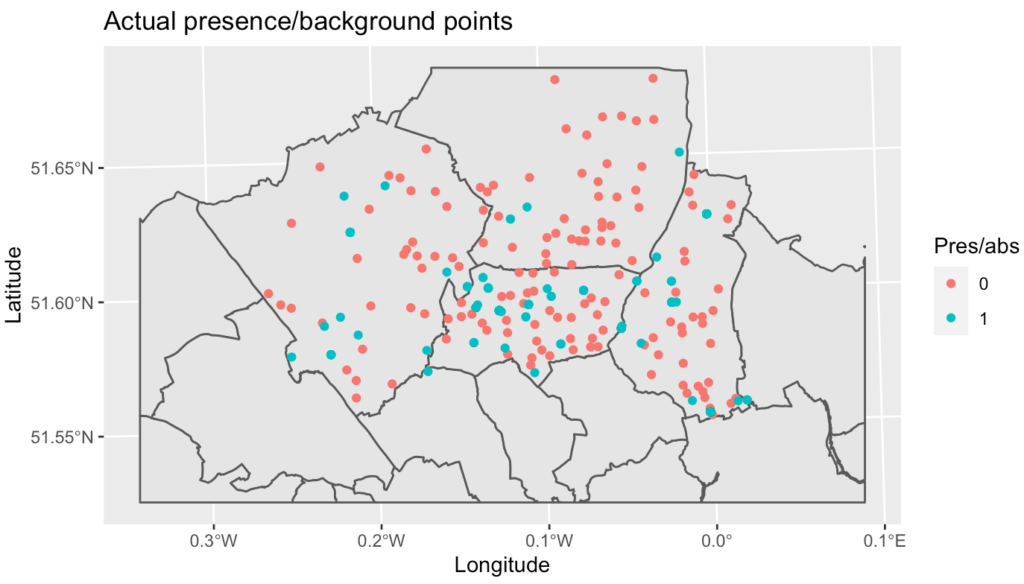
This study was a great starting point for mapping and predicting geographic species counts using socio-environmental and climate variables, but the complexity of ecosystems means that the predictive power of the tested models is still not good enough for accurate prediction and so a further study will be the fitting of generalised linear mixed effects models, generalised additive mixed effects models and using RJAGS Bayesian techniques. Including possible missing important variables could also help to improve the existing models.
